
So, how does one go about finding a Lyapanov exponent for a system? Sprott describes this well:
The largest Lyapunov exponent of a system can be computed by taking the difference of the current iteration of x(n) and the current iteration of x(n) plus an epsilon, dx(n) , and dividing by the difference of the previous iteration of x(n-1) and previous iteration of x(n-1) + dx(n-1) and taking the natural logarithm. For a large number of iterations N after the attractor settles, sum these values together, then divide by N. Between each iteration, we have to readjust dx(n).Two-dimensional chaotic iterated maps also exhibit sensitivity to initial conditions, but the situation is more complicated than for one-dimensional maps. Imagine a collection of initial conditions filling a small circular region of the XY plane. After one iteration, the points have moved to a new position in the plane, but they now occupy an elongated region called an ellipse. The circle has contracted in one direction and expanded in the other. With each iteration, the ellipse gets longer and narrower, eventually stretching out into a long filament. The orientation of the filament also changes with each iteration, and it wraps up like a ball of taffy.
Thus two-dimensional chaotic maps have not a single Lyapunov exponent but two - a positive one corresponding to the direction of expansion, and a negative one corresponding to the direction of contraction. The signature of chaos is that at least one of the Lyapunov exponents is positive. Furthermore, the magnitude of the negative exponent has to be greater than the positive one so that initial conditions scattered throughout the basin of attraction contract onto an attractor that occupies a negligible portion of the plane. The area of the ellipse continually decreases even as it stretches to an infinite length.
There is a proper way to calculate both of the Lyapunov exponents. For the mathematically inclined, the procedure involves summing the logarithms of the eigenvalues of the Jacobian matrix of the linearized transformation with occasional Gram-Schmidt reorthonormalization. This method is slightly complicated, so we will instead devise a simpler procedure sufficient for determining the largest Lyapunov exponent, which is all we need in order to test for chaos.
[Sprott, pp54-55]
                1   N      dx(n+1)
    λ =  lim   ---  Σ  ln( ------- )
        N->inf  N  n=1      dx(n)
So, what are we actually doing in this process? Consider two close points at time step n, x(n) and x(n)+dx(n). At the next time step they will have diverged to x(n+1) and x(n+1)+dx(n+1). The Lyapunov exponent (traditionally represented by λ) captures the average rate of convergence or divergence. The exponent tells us the rate that we lose information about the initial conditions.
The value of λ tells us information about the attractor:
As I mentioned earlier, between each iteration we must readjust the starting point for x(n)+dx(n). What we want is for x(n)+dx(n) to be readjusted so its separation is the same distance apart as it was before the previous iteration, but in the same direction that dx(n) was from x(n) after the current iteration.
Visually, this looks like:
Remember our questions from above? Well, not only does the Lyapunov exponent tell us if a system is chaotic, it also gives us a measure of how chaotic it is - generally, the further above zero λ is, the more chaotic the system!
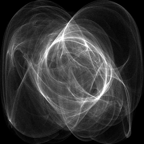
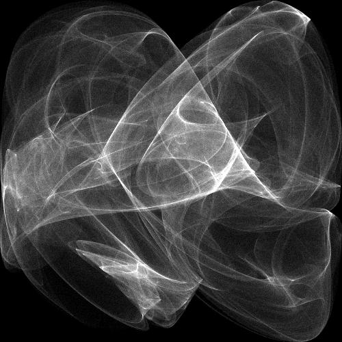
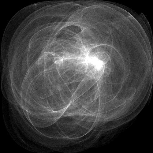
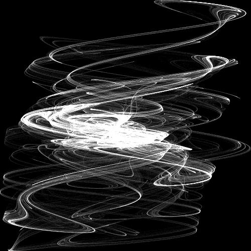
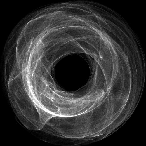
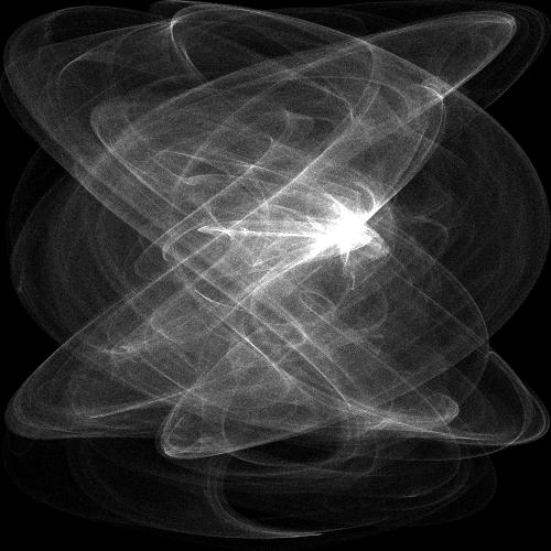
The program lyapdemo.c demonstrates this technique, and saves greyscale images in the PGM format. It is a rewrite of Paul Bourke's Random Attractor program to use the same attractor I had set up previously, and to work more the way I thought it should.
Here are some sample images from a single run of the above program. Some
interesting things to note: Each image is 500x500 pixels and was created
from a 10,000,000 point generation of the attractor. Yes, 10 million
points. It took about 5 minutes to find 10 attractors on an Intel-P4 1.5Ghz,
and the program used a bit over 120MB RAM.
 |
 |
 |
 |
 |
 |
At this point, I have completely rewritten the original program of 1994 to be very modular and dynamically pluggable, in terms of being able to run many attractor types and use many output options, from 2d monochrome and color to 3d renderings. My next move is to add a "movie" option that sits between the attractor generator and the renderer - since I designed the program with this as a future direction, this won't be hard, I just need the time to do it.
This article isn't done yet. I keep adding to it as time allows!
Last updated on 2003-Jan-07