A "Strange" Adventure

The Quest Begins
Way back in the day (well, 1994), my friend Paul and I decided we wanted to visualize three dimensional strange attractors in a realistically shaded way. We had seen a strange attractor or two (in one of Clifford Pickover's books and here and there in other literature, for instance, the famous Lorenz Attractor(1963) and Hénon Attractor (1976)), but all computer-generated pictures we had seen were simple 2-dimensional cross sections. So, we set out to find a way to render an attractor.

We started out by emitting small sphere primitives into a POVRay file and raytracing it. We figured this would work, after all, we had a hot new DEC Alpha 200Mhz UNIX box with 32MB RAM, who could stop us?

Dead End Road
Well, nine thousand scant primitives and three hours later, we got our first picture. And swiftly we realized from our system analysis that we didn't have enough memory (or years) to wait to be able to run the five million primitives per attractor that we desired to get very nice images. We also realized that we had no idea how to add a body of zero dimension (a point cloud) into a raytracer as a primitive type that could be hit by light rays, preventing our hacking up the source to POVRay. In fact, I doubt it is possible. So, it was back to the drawing board.

The Road Already Travelled
We started reading some texts, and deep in Foley, vanDam, Feiner, & Hughes we discovered something called the "Z-Buffer Algorithm". Certain this solution would please even Jon Bentley, we set out to implement a point cloud raytracer using two Zbuffers, one for the camera view, and one for shadows. Before we finished, we discovered something amazing... Tim Stilson, out at Stanford, had beat us to the punch. His images were the most amazing things we had ever seen. However, rather than get (too) discouraged, we were happy to see we were on the right track - Tim's algorithm also used a Zbuffer!

Reaching Base Camp
Within another week or two, we had produced our very first strange attractor rendering. While it has been lost to the mists of time, the image below is our second image. We didn't have color implemented, and we didn't really have a lighting model that was worth anything, but we had pictures, and they didn't take forever to create, in fact, rendering a five million point attractor took about two-and-a-half minutes on the Alpha - we were happy!

The Mountain Becomes Trecherous
Now that we could make pictures, we could go about exploring attractor space! We improved the lighting model by adding diffuse, ambient, and specular lighting, and started rendering up a storm. Here are our results from that time:

Unfortunately, while these images were pretty nice, they took us hours and hours to find. You see, the original equations were we using for our attractors were, like any attractor, highly dependant on the initial conditions of the equations. And worse, most of the initial conditions we tried were not good chaotic attractors - we either got total divergence (no attractor) or a fixed-point attractor (two to twelve pixels colored in) most of the time. Let us perform our own little gedanken experiment.

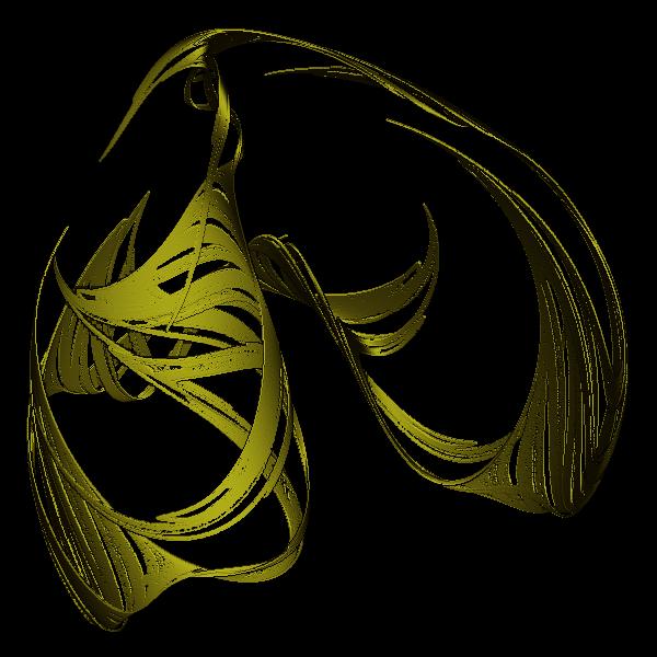
In The Mountains of Madness
To start our experiment, we need to look at the equations in question:

	x'	= sin(Ay) − z cos(Bx)
	y'	= z sin(Cx) − cos(Dy)
	z'	= E sin(x)

What these equations state is that to get the next value for the x-coordinate, you need to take the sine of a constant, A, times the current value for the y-coordinate and subtract the cosine of a constant, B, times the current value for the x-coordinate. The new y and z values are computed similarly.

"But wait!", I hear you say. "How to you pick the first x, y, and z? How do you pick the first A, B, C, D, and E?" Well, calm down. It isn't that hard.

In general, you pick x, y, and z from anywhere within the basin of attraction for your attractor. If in doubt of being in the basin (and we are, by the way), we just want to pick a point near (0,0,0). In fact, we pretty much always used zero back then. And the constants are chosen randomly - we mostly looked at ones in the range of [−1.7, 2.24]. So, lets pick a set at random:

	A	2.0
	B	0.5
	C	−1.0
	D	−1.0
	E	2.0

Now let's start running the equation, over, and over, and over again:
(You can play along too, if you have a C compiler: attr.c)

iter	x	y	z
0	0.000000	0.000000	0.000000
1	0.000000	−1.000000	0.000000
2	−0.909297	−0.540302	0.000000
3	−0.882243	−0.857553	−1.578145
...
112	−1.918912	1.053076	−1.834793
113	1.913196	−2.219638	−1.880034
114	2.046407	2.375166	1.883904
115	−1.980104	−0.954422	1.778027
116	−1.918912	1.053076	−1.834793
117	1.913196	−2.219638	−1.880034
118	2.046407	2.375166	1.883904
119	−1.980104	−0.954422	1.778027

As you can see, iterations 112 through 115 are repeated in iterations 116 through 117 in a four point cycle, making this a fixed point attractor with four fixed points. While this is pretty nifty from a mathematical standpoint, this is not going to make any pretty pictures. So we have before us some interesting questions:
· How does one go about finding out if a given attractor is chaotic?
· How does one go about measuring not just if an attractor is chaotic, but how chaotic it is?

Storm in the Mountains
Paul managed to find a few more attractors using nothing more than elbow grease and will. Here are his images from this time:

About this time, we stopped working on the project - Paul was deeply involved with DNA research and his graduate studies and I was busy finishing my degree, graduating, moving, and working hard at my new job. We were not sure we would ever find a "real" answer to our questions.

Resuming the Traverse
Walking through the bookstore one day in Southern New Mexico, I ran across a very cool book... One referenced on Tim Stilson's page, although I had never bothered looking it up. The book was Strange Attractors: Creating Patterns in Chaos by Julien C. Sprott. (This book is out-of-print, however, you can download (8MB) a PDF file of the book from Dr. Sprott, who has graciously made it available on the web!)

I was busy, the book sat on my shelf until 1999, when I picked it up and played with the software on the floppy that came with the book (Yes, it is still on Dr. Sprott's site). I became apparent that there was a way of answering the above questions, as the software did searches for attractors that were pretty successful. Even though I was busy, I became addicted to the 3d attractors of the interlocked quadratic map equations and decided to modify our now-old program to handle these beauties. So, I turned to Appendix E where all the equations were, found this equation:



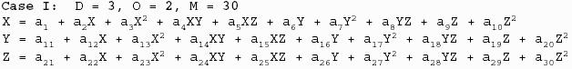
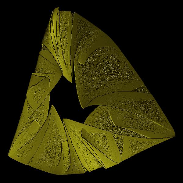
And promptly added it with its thirty parameters to the codebase and made images from the file SA.DIC supplied with the book. Mind you, I didn't really read the book, I just typed in the equation and made the following pictures:

Approaching the Apex
I mailed the changes to Paul, and life became busy again. But before Christmas in 2001, I decided it would be fun to revamp some of the old code. I looked for it. And then I looked some more. Somehow, I had failed to keep even one copy of the program around. I sent an urgent mail to Paul and thankfully, he had kept the last set of changes. This proved enough for me, I saved the code in about twenty places and didn't even get around to trying to compile it until the next May.

I was sitting in my family room contemplating what to read next after having finished Jostein Gaardner's "The Solitaire Mystery" (good, although I liked "Sophie's World" even more) and, Sprott's book caught my eye. I sat down, and began reading. I had heard about the Lyapunov exponent being able to find whether or not attractors were chaotic, and in Sprott's book I began to understand how to go about computing these values, more importantly, the value of the largest Lyapunov exponent of a system, which is the only one needed to be able to tell if an attractor is chaotic. So, I set out to code up my own Lyapunov attractor finder.

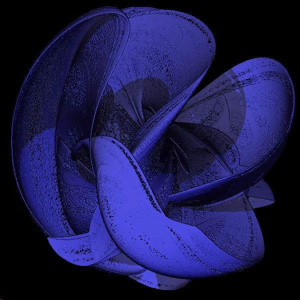
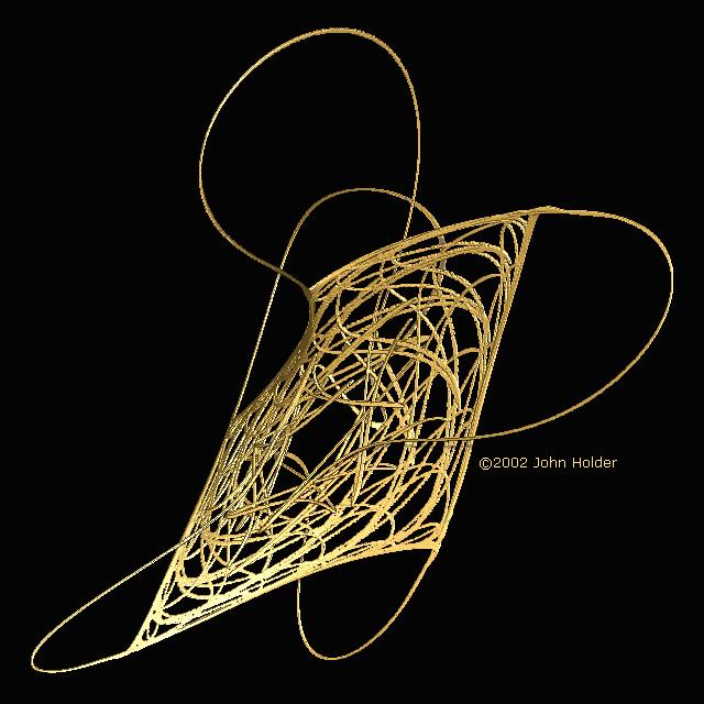
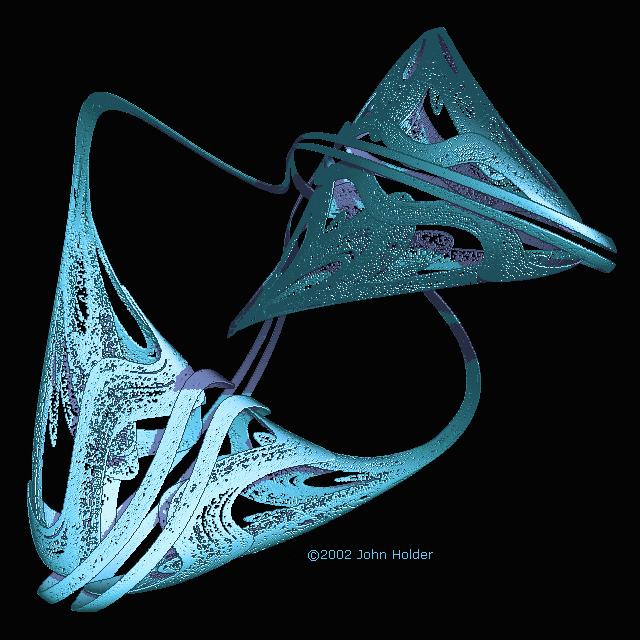
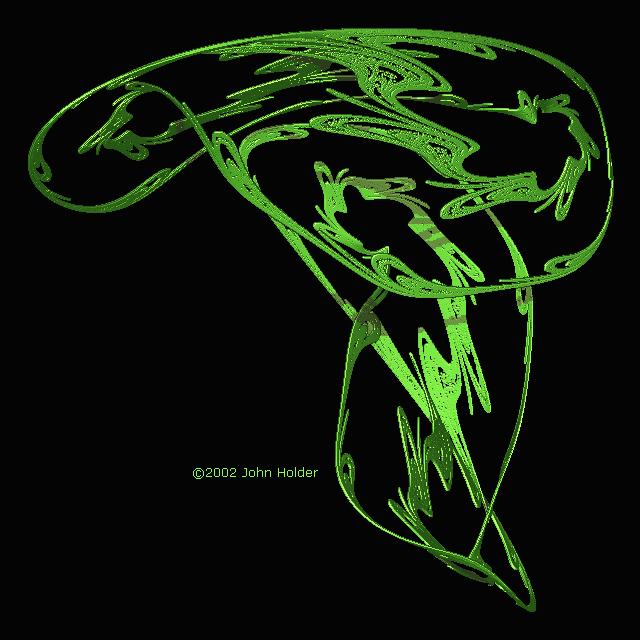
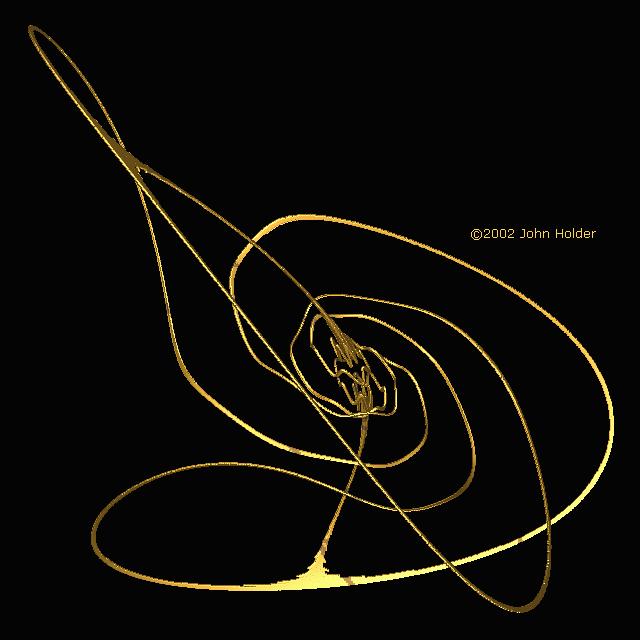
However, before that happened, I got distracted - I noticed something inside our lighting model that I felt compelled to fix - I added a parameter that, when any one color value is increased into what formerly would have been an overflow situation, the other color components are brightened in a ratio consistent with the lamp color. This had the effect of greatly improving the quality of the images. I also discovered that most of our images needed to be seriously gamma corrected! So, before writing a Lyapunov attractor finder, I made these pictures: (NOTE: The pictures start getting really good here!)
As the above images demonstrate, perhaps amusingly, we had achieved our original goal, to visualize three dimensional strange attractors in a realistically shaded way. However, we had not achived the now more important goal of answering our questions.

---

Copyright © 2003 by John Holder